Q1. What is the Black Scholes Model?
The Black-Scholes model is a mathematical model used for pricing options contracts. It was developed by Fischer Black, Myron Scholes, and Robert Merton in the early 1970s and has become a foundational tool in the field of quantitative finance. This model helps determine the theoretical price of European-style options, considering various factors that affect option pricing.
The primary use of the Black-Scholes model is to calculate the fair market value of options based on several variables, including: strike price, underlying stock price, expiration date, risk free interest rate, and volatility.
It’s important to note that while the Black-Scholes model is widely used, it has certain limitations, including assumptions that might not always hold true in real-world market conditions, such as constant volatility and no dividends.
Q2. What are the assumptions underlying the Black Scholes Model?
Following are the assumptions of Black Scholes Model:
1) European-style options: The Black-Scholes model is specifically designed for European-style options, which can only be exercised at expiration.
2) Log-normal distribution of stock prices: It assumes that the price movement of the underlying asset follows a log-normal distribution.
3) Constant volatility: The model assumes that the volatility of the underlying asset’s returns remains constant throughout the option’s life.
4) Efficient markets: The model operates under the assumption that markets are efficient and that there are no arbitrage opportunities available.
5) Constant risk-free interest rate: The model assumes a constant risk-free interest rate for the entire life of the option.
6) No dividends: The model assumes that the underlying asset doesn’t pay any dividends during the option’s life.
Q3. What are the components of the Black Scholes Model?
The Black-Scholes formula consists of 5 components
- S – Current Stock Price: This is the current market price of the underlying asset (e.g., stock, index).
- K – Strike Price: It’s the predetermined price at which the holder of the option can buy or sell the underlying asset.
- T – Time to Expiration: This represents the time remaining until the option contract expires. It’s usually measured in years.
- r – Risk-Free Interest Rate: This is the interest rate of a risk-free investment, like a government bond, for the duration of the option. It’s an annualized rate.
- σ – Volatility: Volatility measures the fluctuation in the price of the underlying asset. In the Black-Scholes model, volatility is assumed to be constant for the duration of the option.
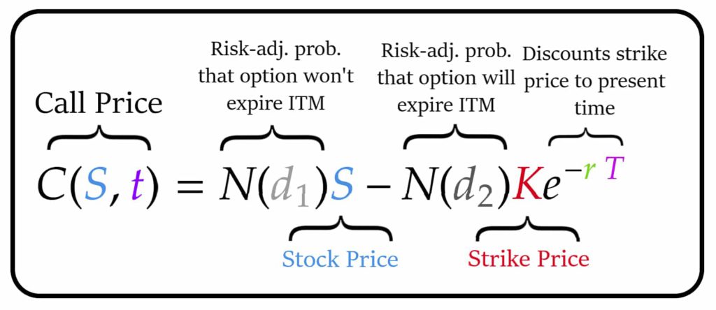
Q4. What is the formula of the Black-Scholes Model?
The Black-Scholes formula for pricing a call and put option is given by:


Q5. How does volatility affect option price of the Black Scholes Model?
Volatility has a direct impact on option prices. Higher volatility leads to higher option prices movement (both call and put options). When volatility increases, the potential for the underlying asset’s price to move significantly in either direction also increases which in turn can lead to profits. This makes the option more valuable, leading to higher option premiums.
Overall, in the Black-Scholes framework, volatility is a critical factor influencing option prices. Higher volatility leads to higher option premiums, reflecting the increased uncertainty and potential for larger price movements in the underlying asset.
However, it’s essential to note that this relationship assumes constant volatility over the option’s life, which might not always hold true in real markets.
Q6. What are some alternative models or modifications to the Black-Scholes model used in option pricing?
Several alternative models and modifications to the Black-Scholes model have been developed to address its limitations. Some of these include:
- Binomial Options Pricing Model (BOPM): This model is based on a discrete-time framework and allows for multiple periods before the option’s expiration. It’s more flexible than Black-Scholes as it can handle a variety of assumptions about dividends, interest rates, and volatility changes over time.
- Heston Model: This stochastic volatility model introduces volatility as a random process that evolves over time. It addresses one of the key limitations of the Black-Scholes model by allowing volatility to fluctuate, reflecting real-world market conditions more accurately.
- Jump Diffusion Models: These models incorporate occasional large price movements or jumps in the underlying asset’s price, which are not accounted for in the Black-Scholes model. They combine continuous diffusion processes (representing normal price movements) with occasional jumps.
- Jump Diffusion Models: These models incorporate occasional large price movements or jumps in the underlying asset’s price, which are not accounted for in the Black-Scholes model. They combine continuous diffusion processes (representing normal price movements) with occasional jumps.
- Variance Gamma Model: This model captures both stochastic volatility and jumps in asset prices. It introduces a gamma process to account for jumps in prices, aiming to improve accuracy when dealing with large price movements.
- Stochastic Interest Rate Models: Some models incorporate stochastic interest rates, as opposed to assuming a constant risk-free rate. These models aim to better capture the dynamics of interest rates, which can significantly impact option pricing.
Q7. What are the risk measures used in Option Trading?
The Greeks which is referred as risk measures or sensitivities are used the in options trading and risk management. They are derived from mathematical models like the Black-Scholes equation and provide insights into how an option’s price is influenced by various factors. Here’s an overview of the main Greeks:
1) Delta (Δ): Delta measures the change in an option’s price in relation to changes in the price of the underlying asset. It indicates the sensitivity of the option’s price to movements in the underlying asset price.
2) Gamma (Γ): Gamma measures the rate of change of an option’s delta concerning changes in the underlying asset price. It indicates how much the delta might change as the underlying asset price changes.
3) Theta (Θ): Theta measures the change in an option’s price due to the passage of time. It shows how much the option’s price might decrease as time passes, capturing the effect of time decay.
4) Vega (V): Vega measures an option’s sensitivity to changes in implied volatility. It quantifies how much an option’s price might change for a one-percentage-point change in volatility.
5) Rho (ρ): Rho measures an option’s sensitivity to changes in the risk-free interest rate. It indicates how much an option’s price might change for a one-percentage-point change in the risk-free interest rate.